Options Valuation Model

MesoSim's Options Valuation Model projects option PnL and Greeks at a chosen time and underlying price. Use these values in strategy filters, adjustments, and exit rules, or to identify points on a Risk Graph. Available with Advanced and FundPro; see Accounts and Access.

• options.model evaluates one scenario, such as projected PnL after five days if the underlying falls 2%.
• options.model_solver searches a price range for a minimum, maximum, or candidate zero crossing, such as a break-even price.

The calculations use the selected legs' current Implied Volatility and the pricing model appropriate to the contracts. They describe a scenario at the chosen horizon, rather than forecasting future prices or volatility. See Position Monitor for visual exploration of projected risk.

Evaluate one scenario

For a position that has already been selected, this expression projects PnL five calendar days from the current simulation time at an underlying price 2% below its current value:

options.model(position, 5, underlying_price * 0.98, pnl)

The second argument is days forward from now, including fractions. It is not the desired remaining DTE: 0 means now, 0.5 means twelve hours from now, and 5 means five days from now.

Use the expression in Entry.VarDefines, or in an adjustment or exit expression with the required position context. Entry.Conditions runs before leg selection; use Entry.AbortConditions for an entry filter based on the selected position's projected values.

Practical example

For a calendar structure, search the projected PnL curve at its first expiration for lower and upper break-even candidates and its highest and lowest values within a chosen price range.

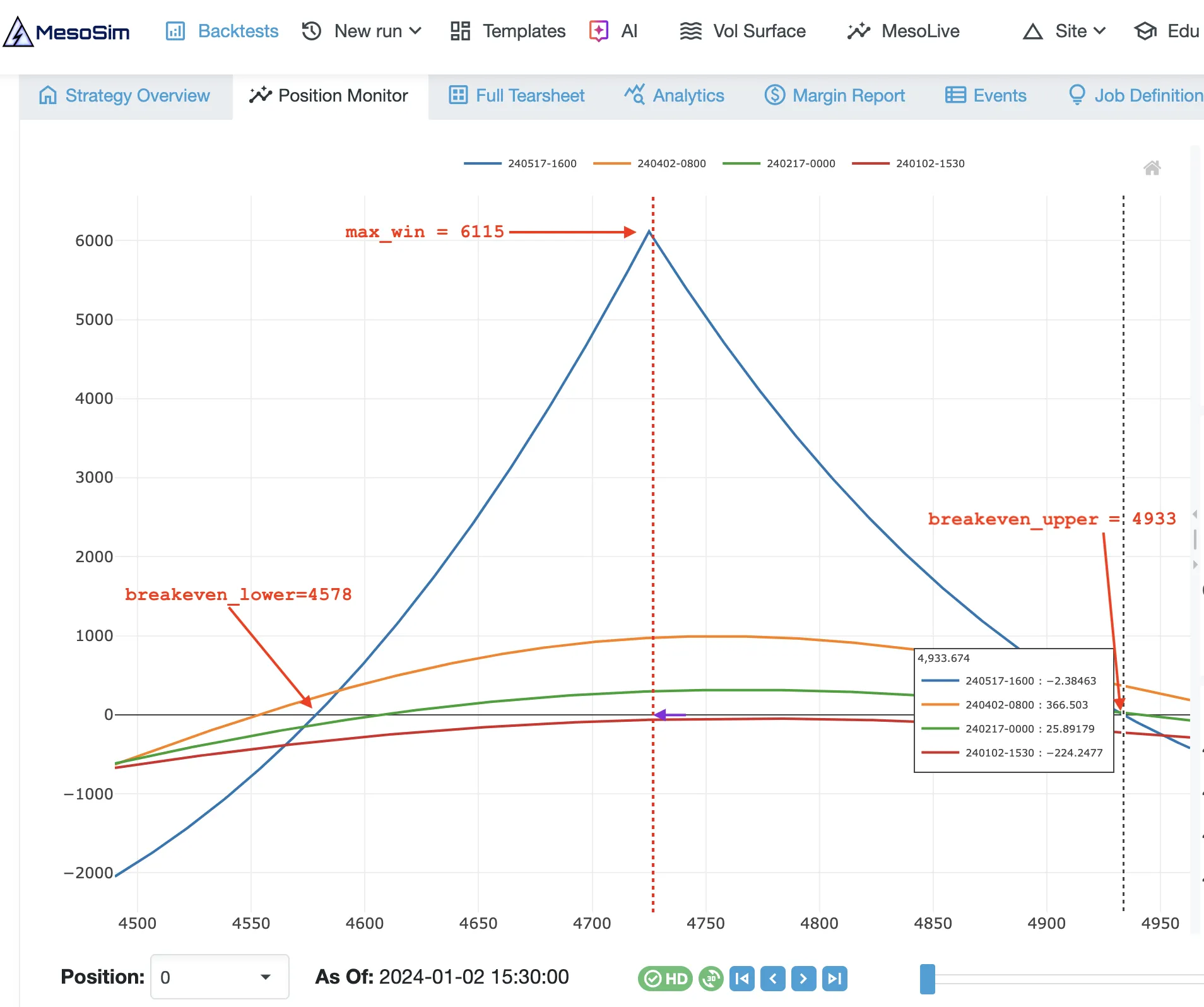
Merge this fragment into your strategy, keeping its structure, schedules, and other required fields:

{
  "Entry": {
    "VarDefines": {
      "breakeven_lower": "options.model_solver(position, first_exp, underlying_price * 0.5, underlying_price * 2, pnl, zero, return_price)",
      "breakeven_upper": "options.model_solver(position, first_exp, underlying_price * 2, underlying_price * 0.5, pnl, zero, return_price)",
      "projected_max_pnl": "options.model_solver(position, first_exp, underlying_price * 0.5, underlying_price * 2, pnl, maximize, return_value)",
      "projected_min_pnl": "options.model_solver(position, first_exp, underlying_price * 0.5, underlying_price * 2, pnl, minimize, return_value)"
    }
  }
}

The first search scans from low to high prices; the second reverses the direction to find a crossing from the other side. They identify different break-even points only when the curve has suitable crossings within the range. The maximum and minimum describe this range and horizon, not the strategy's unlimited-price or lifetime risk.

Verify a break-even candidate

A returned price alone does not establish a break-even point. Check it with options.model using the same target, horizon, and metric, and verify that PnL is close to zero. Compare the curve on either side if you need to confirm a crossing.

Inspect the captured values in the Events Viewer and compare them with the corresponding Risk Graph in Position Monitor. The [FEAT-OptionValuation] built-in template demonstrates this type of analysis; the example above uses first_exp to state the horizon explicitly.

Prefer a single-point evaluation when possible

options.model evaluates one price. Use options.model_solver when you need to search a range; repeated searches increase simulation time.

Module prototypes

Functions

Signature	Description
options.model(target, dteDaysOrAnchor, underlyingPrice, metric[, model_params]) -> number or nil	Evaluate position/leg at a time anchor or a number of days from now using a scenario underlying price and return the selected metric
options.model_solver(target, dteOrKey, start, end, metric, goal, result[, solver_params]) -> number or nil	Scan a price range to minimize/maximize/zero a metric and return value or price per result

Targets

Name	Description
position	Evaluate the position’s open option legs, or its selected pending legs before entry
leg_<name>	Evaluate a specific option leg by name, such as leg_short_call

Time Anchors

Name	Description
at_exp	Earliest expiration among the selected legs; same horizon as first_exp
first_exp	Earliest expiration among the selected legs
last_exp	Latest expiration among the selected legs
now	Current backtest time (numeric horizon 0)

Metrics

Name	Description
pnl	Projected PnL of the evaluated legs
delta	Sensitivity to underlying price
gamma	Rate of change of delta
theta	Time decay
vega	Sensitivity to volatility
wvega	Weighted vega using option DTE
rho	Sensitivity to interest rates

Goals

Name	Description
minimize	Find the minimum of the metric over the price range
maximize	Find the maximum of the metric over the price range
zero or root	Search for a zero crossing of the metric

Result

Name	Description
return_value	Return the metric value at the solution
return_price	Return the underlying price at the solution (alias: strike)
strike	Alias for return_price

Parameters at a Glance

• target: position or leg_<name>
• dteDaysOrAnchor / dteOrKey: non-negative days from the current simulation time or a time anchor (at_exp, first_exp, last_exp, now)
• metric: one of pnl, delta, gamma, theta, vega, wvega, rho
• goal: minimize, maximize, zero, or its alias root (for solver)
• result: return_value or return_price/strike (for solver)
• underlyingPrice, start, and end: positive underlying prices, not option strike selections
• model_params: reserved; omit it
• solver_params: optional Lua table with steps, an integer from 1 to 500; default 500

The target, anchor, metric, goal, and result names are Lua keywords: write position, pnl, and first_exp without quotes. Replace leg_<name> with a leg name from your strategy.

The model includes quantity, direction, and contract multiplier. An individual marker leg is evaluated as if its quantity were 1, in both options.model and options.model_solver; marker legs contribute zero when the target is position. Projected PnL describes the evaluated legs relative to their entry prices; it does not add realized PnL from previously closed legs. Legs that expire before the chosen horizon are excluded, so last_exp does not reconstruct the complete lifecycle of a multi-expiration position.

Solver resolution

For example, request 200 price-grid steps with an optional Lua table:

options.model_solver(position, first_exp,
  underlying_price * 0.8, underlying_price * 1.2,
  pnl, maximize, return_price, { steps = 200 })

More steps give a finer grid over the same range and require more calculation. Solver results are numerical estimates within that range. Choose a relevant range and verify important values with options.model and the Risk Graph.

Usage Notes

• Use an available target. Position and leg evaluations require selected or open options. See Variable availability.
• Check unavailable results. A calculation can return nil when required valuation data is unavailable. Check availability before using a result in arithmetic or a comparison; do not interpret an unavailable calculation as zero PnL.
• Keep the horizon consistent. Compare model and Risk Graph values at the same time, underlying price, and position state.
• Choose scan direction deliberately. Reversing start and end reverses the zero-crossing search. It does not expand the search range.

Write and validate expressions in the AI Job Editor. See Strategy Definition Reference for the fields that accept them, and the Deltaray blog for full strategies with analysis.